Why RC Curves Are Exponential

Branch role: This optional enrichment page gives the calculus reason for the exponential RC curves used in Capacitor Networks and RC Switching.

Further enrichment outside active 9749

The entire capacitance dossier lies outside the active 9749 syllabus. This optional branch goes further by using differential equations to derive the simple ideal RC formulae.

Overview

The simple RC equations are exponential because the rate of change of charge is proportional to the remaining difference from the final state. This derivation is included for students who want the reason behind the curves; it is not active 9749 core content.

Core Ideas

• Discharge gives a rate equation proportional to the present charge.
• Charging gives a rate equation proportional to the remaining uncharged fraction.
• The time constant $\tau =RC$ sets the scale over which the difference from the limiting value changes by a factor of $e$.

Exam Relevance

Use this note only as enrichment. For ordinary capacitor-switching questions, the safer operational skill is applying the given exponential equations and stating their model assumptions.

Model and sign convention

The derivations below apply only to a circuit containing one ideal capacitor of constant capacitance $C$ and one constant resistance $R$. The source, connecting wires and switch are ideal, and capacitor leakage is neglected.

Let $Q(t)\ge 0$ be the magnitude of charge on either capacitor plate. Then

$$V_C=\frac{Q}{C}.$$

The signed current depends on the chosen reference direction. To avoid hiding that choice, this note writes $|I|$ for current magnitude:

• during discharge, $Q$ decreases, so $|I|=-dQ/dt$;
• during charging, $Q$ increases, so $|I|=dQ/dt$.

The common mathematical structure is

$$\frac{dx}{dt}=-kx,$$

whose solution is exponential decay. In an RC circuit, the decaying quantity is either the charge still present during discharge or the charge still missing during charging.

Discharging through a resistor

Suppose the initial charge magnitude is $Q_0$ and the initial capacitor p.d. is $V_0=Q_0/C$. At any later time, the resistor p.d. equals the capacitor p.d. in magnitude:

$$|I|=\frac{V_C}{R}=\frac{Q}{RC}.$$

Because $Q$ is decreasing,

$$-\frac{dQ}{dt}=\frac{Q}{RC},$$

or

$$\frac{dQ}{dt}=-\frac{Q}{RC}.$$

Separating variables and integrating gives

$${\int }_{Q_0}^Q\frac{d{Q}^{\prime }}{Q^{\prime }}=-{\int }_0^t\frac{d{t}^{\prime }}{RC},$$

so

$$\ln \left(\frac{Q}{Q_0}\right)=-\frac{t}{RC}$$

and therefore

$$Q(t)=Q_0{e}^{-t/RC}.$$

Since $V_C=Q/C$ and $|I|=Q/(RC)$,

$$V_C(t)=V_0{e}^{-t/RC},|I(t)|=\frac{V_0}{R}{e}^{-t/RC}.$$

The current direction is the discharge direction; the equation above gives only its magnitude.

Charging from an ideal source

Now connect an initially uncharged capacitor to a constant source p.d. $V_s$ through $R$. During charging, Kirchhoff’s loop rule gives

$$V_s=|I|R+V_C.$$

Using $|I|=dQ/dt$ and $V_C=Q/C$,

$$V_s=R\frac{dQ}{dt}+\frac{Q}{C}.$$

Hence

$$\frac{dQ}{dt}=\frac{C{V}_s-Q}{RC}.$$

The final charge magnitude is $Q_{\infty }=C{V}_s$. Define the missing charge

$$u=Q_{\infty }-Q.$$

Then

$$\frac{du}{dt}=-\frac{u}{RC}.$$

Because the capacitor is initially uncharged, $u(0)=Q_{\infty }$. Therefore

$$u=Q_{\infty }{e}^{-t/RC},$$

which gives

$$Q(t)=C{V}_s\left(1-e^{-t/RC}\right).$$

The capacitor p.d. and current magnitude are

$$V_C(t)=V_s\left(1-e^{-t/RC}\right),|I(t)|=\frac{V_s}{R}{e}^{-t/RC}.$$

Thus $V_C$ rises toward $V_s$, while the current magnitude falls from $V_s/R$ toward zero.

Interpreting the time constant

The time constant is

$$\tau =RC.$$

Its unit is seconds because

$$\Omega \mathrm{F}=\frac{\mathrm{V}}{\mathrm{A}}\frac{\mathrm{C}}{\mathrm{V}}=\frac{\mathrm{C}}{\mathrm{A}}=\mathrm{s}.$$

After one time constant:

• a decaying fraction is $e^{-1}\approx 0.368$;
• a rising fraction is $1-e^{-1}\approx 0.632$.

After five time constants, the decaying fraction is $e^{-5}\approx 0.0067$. The capacitor is therefore approximately, not exactly, at its final state.

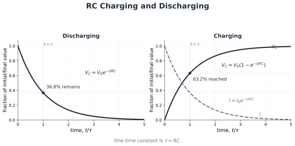
Figure: Exact normalized exponential functions for the simple ideal RC model. In discharge, $V_C/V_0=e^{-t/RC}$ and $|I|/(V_0/R)=e^{-t/RC}$. In charging from zero, $V_C/V_s=1-e^{-t/RC}$ while $|I|/(V_s/R)=e^{-t/RC}$. The curves approach their limiting values asymptotically.

Result map

Process	Quantity that decays as $e^{-t/RC}$	Capacitor p.d.
Discharge from $V_0$	$V_C/V_0$ and $|I|/(V_0/R)$	$V_C=V_0{e}^{-t/RC}$
Charge from zero toward $V_s$	missing fraction $1-V_C/V_s$ and $|I|/(V_s/R)$	$V_C=V_s(1-e^{-t/RC})$

The same time constant appears in both processes because the same ideal $R$ and $C$ set how quickly the relevant difference from the final state changes.

Common Misconceptions

Warning

• $Q$ here is a plate-charge magnitude, not the capacitor’s algebraic net charge.
• $V_s$ is the charging source p.d.; $V_0$ is the initial capacitor p.d. in a discharge problem.
• $|I|$ is a magnitude. A signed current may be negative if its reference direction opposes the actual current.
• The short-circuit and open-circuit descriptions at $t=0^{+}$ and $t\to \infty$ are limiting comparisons, not literal replacements for the capacitor.
• The formulae do not automatically apply to networks with non-constant resistance or capacitance, leakage, or multiple interacting energy-storage elements.

Links

• Electric Capacitance
• Capacitor Networks and RC Switching
• DC Circuits