Oscillations and Simple Harmonic Motion

Topic hub: This is the main overview page for Topic 09. Use it as the starting point, then follow the branch notes for deeper treatment of specific subtopics.

Overview

An oscillation is a repeated to-and-fro variation about an equilibrium position. An ideal undamped oscillation is periodic, so its complete state repeats after equal time intervals. A damped oscillation still moves about equilibrium, but it is not strictly periodic because its amplitude and energy decrease.

Many physical systems oscillate when displaced from equilibrium and released, because a restoring tendency brings the system back while inertia carries it past equilibrium.

Common examples include spring-mass systems, pendulums, vibrating strings, tuning forks, vehicle suspensions, and electrical oscillators.

This hub is the canonical topic page for oscillations and SHM. It is intentionally self-sufficient; the linked pages only expand areas that often need separate treatment.

Core Ideas

• Oscillatory motion repeatedly varies about an equilibrium position; ideal undamped oscillation is periodic.
• A restoring force acts toward the equilibrium position.
• In ideal free oscillation, total mechanical energy remains constant.
• In real systems, dissipative forces such as friction and air resistance cause damping.
• If a periodic external driving force acts on a system, forced oscillations may occur.
• Resonance is identified by the maximum steady-state displacement amplitude as the driving frequency is varied. This occurs at the resonant frequency $f_r$, which is near the undamped natural frequency $f_0$; $f_r\approx f_0$ for negligible or light damping and may lie below $f_0$ when damping is appreciable.

Describing Oscillations

The equilibrium position is the position where the resultant force on the object is zero:

$$\sum \vec{F}=\vec{0}$$

In many JC SHM problems, the motion is treated in one dimension after choosing a positive direction. The displacement $x$, velocity $v$, and acceleration $a$ are then signed components of the underlying displacement, velocity, and acceleration vectors along that chosen line. The sign represents the direction.

The signed displacement $x$ is measured from equilibrium:

• $x>0$: one side of equilibrium that is chosen as positive direction;
• $x<0$: opposite side.

Amplitude $x_0$ is the maximum magnitude of displacement:

$$|x{|}_{\max }=x_0$$

The period $T$ is the time for one complete oscillation. The frequency $f$ is the number of oscillations per second:

$$f=\frac{1}{T}$$

Angular frequency is the scalar rate of phase change:

$$\omega =2\pi f=\frac{2\pi }{T}$$

Phase describes the stage of motion within a periodic cycle.

For any periodic motion or wave with period $T$, a time lag $\Delta t$ corresponds to a phase difference:

$$\Delta \varphi =\frac{2\pi \Delta t}{T}$$

Since one complete cycle corresponds to a phase change of $2\pi$ radians over a time interval $T$,

$$\frac{\Delta \varphi }{2\pi }=\frac{\Delta t}{T}$$

which leads to the above equation.

This comparison applies to two same-frequency oscillations or to two states of one periodic motion. Phase difference is defined modulo $2\pi$; state explicitly which oscillation leads or lags if a signed phase difference is required.

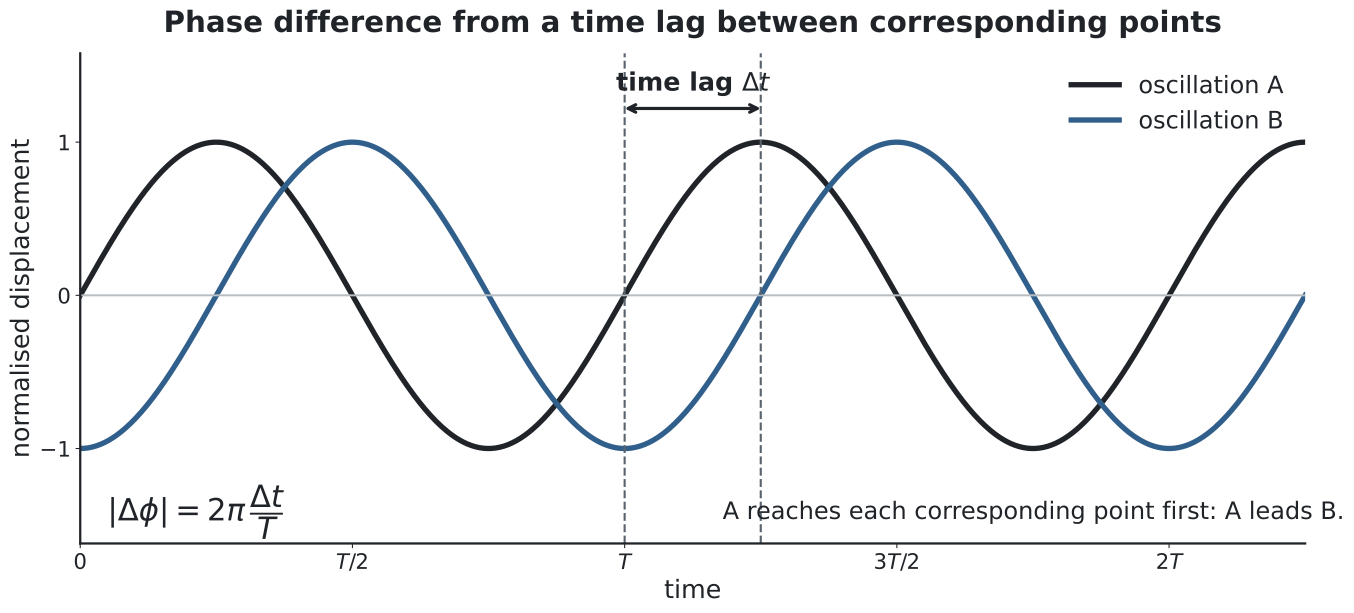
Figure: Measure $\Delta t$ between corresponding points with the same direction of motion, such as successive upward equilibrium crossings. Then $|\Delta \varphi |=2\pi \Delta t/T$; the left-shifted curve leads and the right-shifted curve lags.

Special cases:

• in phase: $\Delta \varphi =0$;
• antiphase: $\Delta \varphi =\pi$.

See Phase Difference.

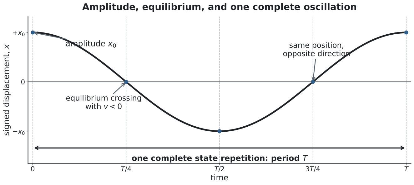
Figure: The equilibrium line is the zero of signed displacement, not a place where the object must be stationary. Amplitude is the greatest value of $|x|$, while the period is the time between two successive states with the same position and direction of motion.

One complete oscillation

A complete oscillation means returning to the same state of motion. Returning to the same position is not always enough: except at a turning point, the object passes a given position twice per cycle, once in each direction.

For example, starting from $x=+x_0$ at rest, one cycle is:

$$+x_0\to 0\to -x_0\to 0\to +x_0.$$

The first and second crossings of $x=0$ are separated by $T/2$, not $T$, because the velocity directions are opposite.

Free Oscillations

A free oscillation occurs when a system is displaced and released, then moves under its own restoring forces without a continuing periodic driver. A real free oscillation may still be damped; free does not necessarily mean undamped.

Examples include a spring-mass system released after displacement, a small-angle pendulum released without a push, and a struck tuning fork after contact with the striker has ended.

Ideal free oscillations have:

• constant amplitude;
• constant period;
• constant total mechanical energy.

Real systems gradually lose energy due to damping.

The natural frequency is the frequency at which the system oscillates when displaced and then left to oscillate freely. It is determined by the physical properties of the oscillator, such as $m$ and $k$ for an ideal spring-mass system. It is not chosen by an external driver.

Simple Harmonic Motion

Simple harmonic motion is oscillatory motion in which acceleration $\vec{a}$ is directly proportional to displacement from equilibrium $\vec{s}$ and always directed toward equilibrium.

Vector form:

$$\vec{a}=-{\omega }^2\vec{s}$$

In the usual one-dimensional signed-component treatment:

$$a=-{\omega }^{2}x$$

The negative sign means acceleration is opposite to displacement:

• if $x>0$, then $a<0$;
• if $x<0$, then $a>0$.

See Simple Harmonic Motion.

Equations of SHM

The displacement can be written as:

$$x=x_0\sin (\omega t+{\varphi }_0)$$

or equivalently:

$$x=x_0\cos (\omega t+{\varphi }_0)$$

depending on initial condition. Here, $\Phi (t)=\omega t+{\varphi }_0$ is the time-varying phase, and ${\varphi }_0$ is the initial phase constant.

Different values of the initial phase ${\varphi }_0$ give the same SHM shape but different starting positions on the displacement-time graph. See Simple Harmonic Motion for worked phase-constant examples.

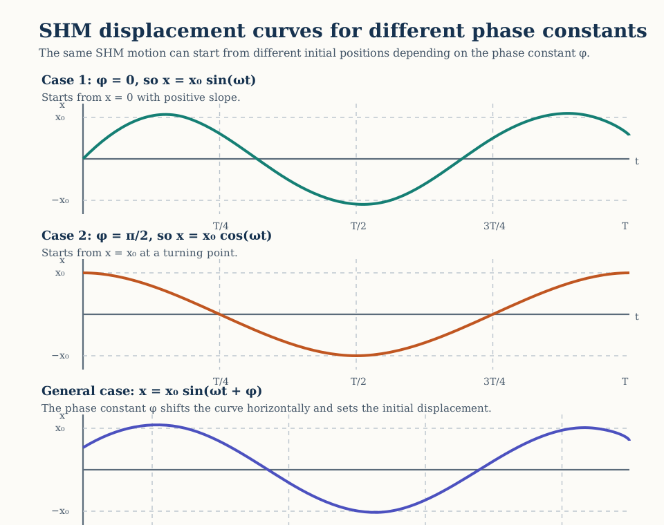
Figure: Changing ${\varphi }_0$ changes the state at $t=0$ but not the amplitude or period. Read both $x(0)$ and the initial slope to distinguish motions that begin at the same displacement but move in opposite directions.

Velocity is:

$$v=\frac{dx}{dt}$$

Here $v$ is the signed velocity component. The speed is $|v|$.

If displacement is written as:

$$x=x_0\sin (\omega t+{\varphi }_0).\text{\hspace{1em}(1)}$$

then differentiating once gives velocity:

$$v=\frac{dx}{dt}=\omega x_0\cos (\omega t+{\varphi }_0).\text{\hspace{1em}(2)}$$

and differentiating again gives acceleration:

$$a=\frac{dv}{dt}=-{\omega }^2{x}_0\sin (\omega t+{\varphi }_0).\text{\hspace{1em}(3)}$$

Comparing (1) and (3), we have:

$$a=-{\omega }^{2}x.\text{\hspace{1em}(4)}$$

The maximum acceleration magnitude is:

$$a_{\max }={\omega }^2{x}_0$$

So the sinusoidal displacement form and the SHM condition are consistent with each other: sinusoidal motion gives restoring acceleration proportional to displacement and directed toward equilibrium.

Displacement, velocity, and acceleration in SHM have fixed phase relationships.

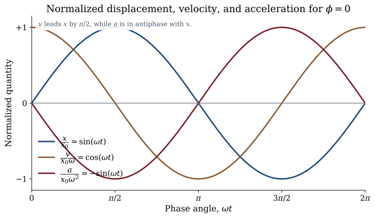
Figure: For $x=x_0\sin \omega t$, velocity leads displacement by $\pi /2$, while acceleration is in antiphase with displacement. The three curves are normalised because their physical units and amplitudes differ.

From (1) and (2) and considering ${\sin }^2(\omega t+{\varphi }_0)+{\cos }^2(\omega t+{\varphi }_0)=1$, we have:

$${\left(\frac{x}{x_0}\right)}^2+{\left(\frac{v}{x_0\omega }\right)}^2=1.\text{\hspace{1em}(5a)}$$

Equivalently,

$$v=\pm \omega \sqrt{x_0^2-x^2}.\text{\hspace{1em}(5b)}$$

The positive and negative signs represent the two possible directions of motion at most positions. Position alone does not determine velocity direction.

Graphical Behaviour in SHM

The displacement-time graph is sinusoidal. It has greatest slope magnitude, and therefore maximum speed, at equilibrium; its slope is zero at the turning points.

The velocity-time graph is also sinusoidal and phase shifted by $\pi /2$ from displacement, so velocity leads displacement by $\pi /2$. Speed is maximum at equilibrium, where $v=\pm \omega x_0$ depending on direction, and velocity is zero at the extremes.

The acceleration-time graph is sinusoidal and in antiphase with displacement.

The acceleration-displacement graph is a straight line:

$$a=-{\omega }^{2}x$$

with gradient:

$$-{\omega }^2$$

This is a common test for SHM. Its range is:

$$-x_0\le x\le x_0,-{\omega }^2{x}_0\le a\le +{\omega }^2{x}_0$$

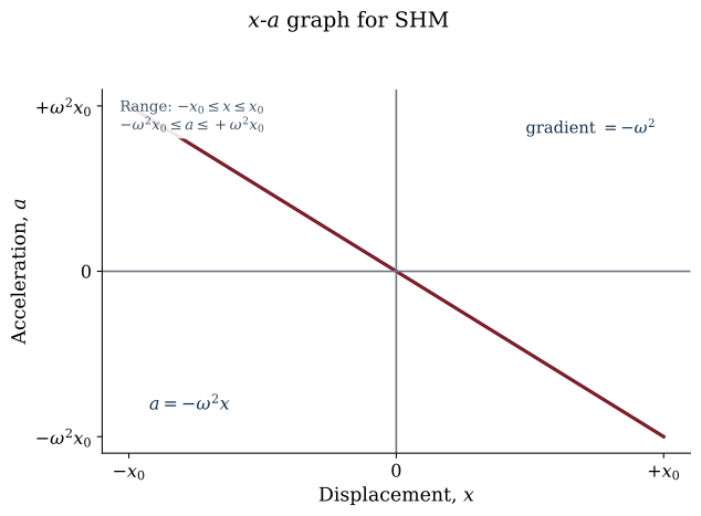
Figure: The $a$-$x$ graph passes through the origin and has constant negative gradient $-{\omega }^2$. This single graph tests both required parts of the SHM definition: proportionality and restoring direction.

The velocity-displacement graph is an ellipse because:

$$v^2={\omega }^2(x_0^2-x^2)$$

Its range is:

$$-x_0\le x\le x_0,-\omega x_0\le v\le +\omega x_0$$

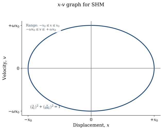
Figure: The upper and lower halves represent motion in opposite directions. At $x=0$, speed is maximum; at $x=\pm x_0$, the object turns around and $v=0$.

Energy in SHM

In ideal SHM, total mechanical energy remains constant.

Kinetic energy is:

$$E_K=\frac{1}{2}m{v}^2.\text{\hspace{1em}(6a)}$$

Using the SHM velocity-displacement relation (5b):

$$E_K=\frac{1}{2}m{\omega }^2(x_0^2-x^2).\text{\hspace{1em}(6b)}$$

The associated potential energy is:

$$E_P=\frac{1}{2}m{\omega }^2{x}^2.\text{\hspace{1em}(7)}$$

A brief derivation of (7):

$$a=-{\omega }^{2}x$$ $$F=ma=-m{\omega }^{2}x$$

where $F$ is the restoring force exerted by the system.

To displace the oscillator slowly from equilibrium to displacement $x$, an external force equal and opposite to the restoring force must be applied:

$$F_{\text{ext}}=-F=m{\omega }^{2}x$$

Hence the potential energy stored is the work done by the external force:

$$E_P={\int }_0^x{F}_{\text{ext}}(x^{\prime })d{x}^{\prime }={\int }_0^{x}m{\omega }^2{x}^{\prime }d{x}^{\prime }=\frac{1}{2}m{\omega }^2{x}^2$$

Total energy is:

$$E_T=E_K+E_P=\frac{1}{2}m{\omega }^2{x}_0^2$$

Equation (6b),

$$E_K=\frac{1}{2}m{\omega }^2(x_0^2-x^2),$$

has a clear physical meaning:

$$E_K=E_T-E_P$$

That is, the kinetic energy at displacement $x$ is the remaining part of the constant total energy after the potential energy $E_P=\frac{1}{2}m{\omega }^2{x}^2$ has been stored.

At equilibrium $x=0$, kinetic energy is maximum and potential energy is minimum. At extremes $x=\pm x_0$, kinetic energy is zero and potential energy is maximum.

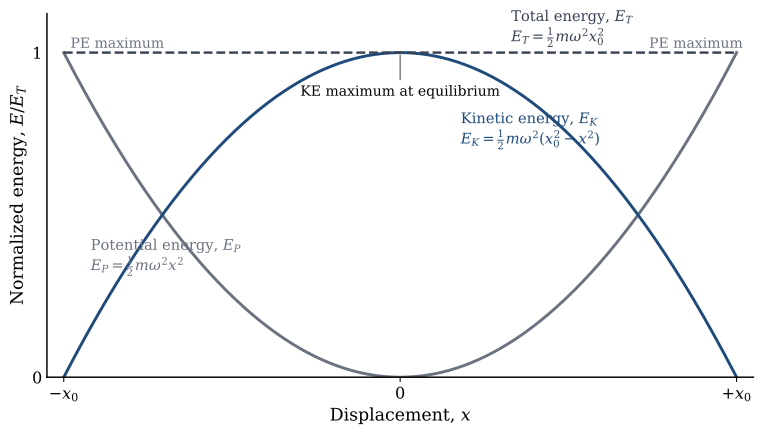
Figure: Against displacement, $E_P$ is an upward parabola and $E_K=E_T-E_P$ is a downward parabola. The vertical separation between $E_T$ and $E_P$ is therefore the kinetic energy, not an additional energy.

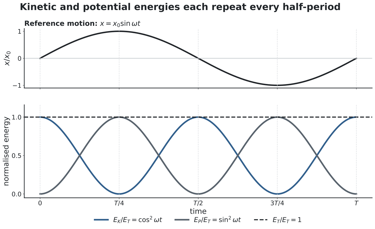
Figure: Against time, $E_K$ and $E_P$ exchange continuously while $E_T$ stays constant. Because the energies depend on squared sine or cosine, each energy repeats every $T/2$, although the displacement repeats every $T$.

State table for one SHM cycle

Position	Velocity	Acceleration	Energy state
$x=+x_0$	$0$	$-{\omega }^2{x}_0$	$E_P$ maximum; $E_K=0$
$x=0$ moving negative	$-\omega x_0$	$0$	$E_K$ maximum; $E_P$ minimum
$x=-x_0$	$0$	$+{\omega }^2{x}_0$	$E_P$ maximum; $E_K=0$
$x=0$ moving positive	$+\omega x_0$	$0$	$E_K$ maximum; $E_P$ minimum

Spring-Mass System

For a horizontal spring:

$$\vec{F}=-k\vec{x}$$

Using Newton’s second law:

$$m\vec{a}=-k\vec{x}$$

Thus:

$$\vec{a}=-\frac{k}{m}\vec{x}$$

Comparing with $\vec{a}=-{\omega }^2\vec{x}$:

$$\omega =\sqrt{\frac{k}{m}}$$

Hence:

$$T=2\pi \sqrt{\frac{m}{k}}$$

This is the cleanest standard SHM example. The key reason it works is that the spring force is a restoring force proportional to displacement from equilibrium. If the mass is pulled to the right, the spring pulls left; if the mass is pushed to the left, the spring pushes right. That is exactly the sign pattern built into:

$$F=-kx$$

and therefore:

$$a=-\frac{k}{m}x$$

So a Hooke’s-law spring implies SHM directly, provided the spring behaves linearly.

Why a Restoring Force Implies SHM

In one-dimensional motion, SHM occurs when the resultant force can be written in the form:

$$F=-kx$$

where $x$ is the signed displacement from equilibrium.

Then Newton’s second law gives:

$$ma=-kx$$

so:

$$a=-\frac{k}{m}x$$

This has exactly the SHM form:

$$a=-{\omega }^{2}x$$

with:

$${\omega }^2=\frac{k}{m}$$

The negative sign matters physically: it means the force and acceleration always point back toward equilibrium. The proportionality matters mathematically: doubling the displacement doubles the restoring acceleration magnitude.

Realistic SHM Models

Several familiar systems become SHM models when the restoring effect is proportional to displacement from equilibrium.

Horizontal Spring-Mass System

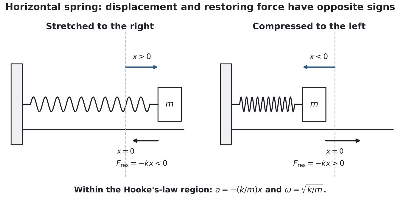
Figure: With right chosen positive, a positive displacement produces a leftward spring force. At equilibrium the resultant is zero, but the mass may pass through with maximum speed.

This is the standard case above. The restoring force is the spring force itself:

$$F=-kx$$

so the motion is SHM.

Vertical Spring-Mass System

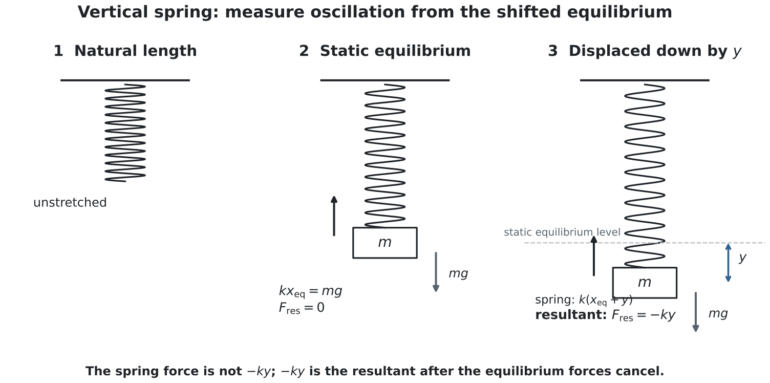
Figure: Weight first produces the static extension $x_{\mathrm{eq}}$. A further displacement $y$ is measured from that equilibrium position; the constant terms cancel, leaving the resultant $F=-ky$.

For a vertical spring, the weight $mg$ changes the equilibrium position but does not destroy SHM. At equilibrium:

$$k{x}_{\text{eq}}=mg$$

If the mass is then displaced by a further small amount $y$ from this equilibrium position, the extra restoring force is:

$$F=-ky$$

because the constant weight is already balanced at equilibrium. So motion about the new equilibrium position is still SHM, with:

$$\omega =\sqrt{\frac{k}{m}}$$

and the same period:

$$T=2\pi \sqrt{\frac{m}{k}}$$

Pendulum at Small Angular Displacement

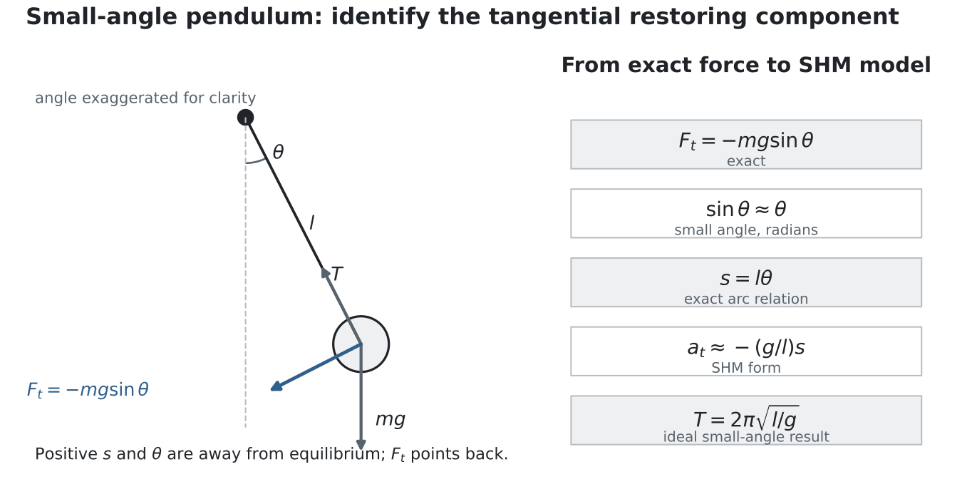
Figure: Tension is radial. The signed tangential component of weight, $-mg\sin \theta$, restores the bob along the arc. Only for small $\theta$ in radians does this become proportional to arc displacement $s=l\theta$.

For a simple pendulum, the tangential restoring force is:

$$F_t=-mg\sin \theta$$

For small angular displacement:

$$\sin \theta \approx \theta$$

and with arc displacement $s=l\theta$, this becomes:

$$F_t\approx -mg\frac{s}{l}=-ks$$

where $k=\frac{mg}{l}$.

So the restoring force is approximately proportional to displacement, which is why small-angle pendulum motion approximates SHM.

Simple Pendulum

For small angular displacement:

$$\sin \theta \approx \theta$$

Then pendulum motion approximates SHM. The angular frequency is:

$$\omega =\sqrt{\frac{k}{m}}=\sqrt{\frac{mg/l}{m}}=\sqrt{\frac{g}{l}}$$

and the period is:

$$T=2\pi \sqrt{\frac{l}{g}}$$

where $l$ is the pendulum length and $g$ is gravitational field strength. The ideal small-angle period is independent of mass.

The simple pendulum formula depends on the small-angle approximation.

See Pendulum Motion.

Floating Partially Immersed Object

A floating object like a cylinder can also oscillate vertically if displaced slightly and released. At equilibrium, upthrust equals weight. Let the vertical displacement from equilibrium be $y=0$ at equilibrium.

If the object is pushed down by a small distance $y$, the immersed volume increases, so the upthrust increases. The extra upthrust acts upward, opposite to the downward displacement.

For a cylindrical rod with cross-sectional area $A$, the extra immersed volume is $Ay$, so the extra upthrust is $\rho gAy$. Since this extra upthrust acts opposite to the downward displacement, the resultant force can be written as:

$$F=-\rho gAy$$

where $\rho$ is the liquid density. Hence, it can be written in a form:

$$F=-ky$$

with $k=\rho gA$. This is again of SHM form:

$$a=-{\omega }^{2}y$$

with $\omega =\sqrt{\frac{k}{m}}=\sqrt{\frac{\rho gA}{m}}$. So a floating, partially immersed object executes SHM for small vertical displacements, provided the cross-sectional area stays effectively constant over the motion.

See Floating Object SHM.

Experimental and Graphical Investigation

Syllabus questions may give displacement-time data from a motion sensor, video tracking, a light gate, or repeated manual timing. A reliable investigation separates measurement from model testing.

1. Measure signed displacement $x$ from the equilibrium position at regular times.
2. Determine $T$ from several cycles and divide by the number of cycles; repeat and average.
3. Obtain velocity from the gradient of the $x$-$t$ graph and acceleration from the gradient of the $v$-$t$ graph, or use suitably processed sensor data.
4. Plot $a$ against $x$.
5. A straight line through the origin with negative gradient supports the SHM model; its gradient equals $-{\omega }^2$.
6. Compare $\omega =\sqrt{-\text{gradient}}$ with $2\pi /T$ as a consistency check.

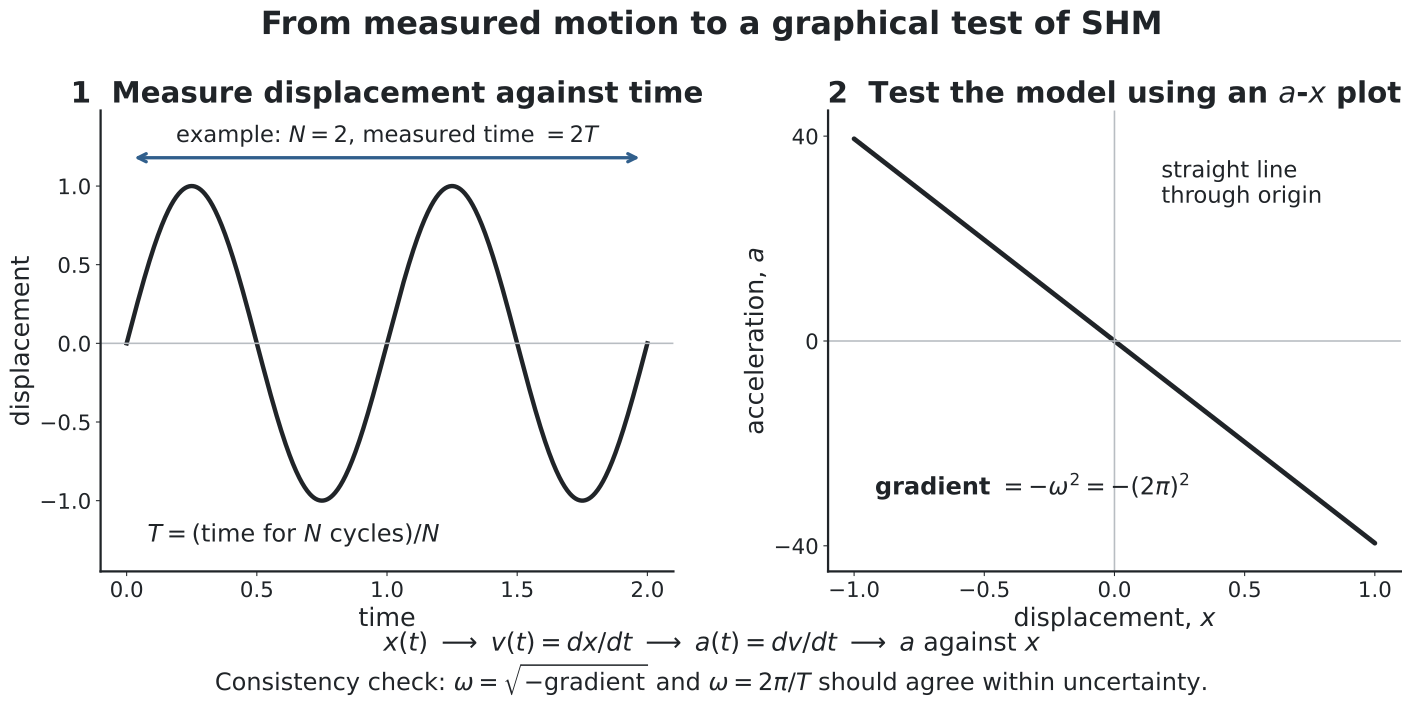
Figure: Time-series measurements yield $x(t)$, then $v(t)$ and $a(t)$. The decisive graphical test is not merely a sinusoidal-looking trace: an $a$-$x$ plot should be a straight line through the origin with negative gradient.

Practical cautions include measuring from the correct equilibrium position, timing many cycles to reduce reaction-time percentage uncertainty, using the same-direction crossing of a fiducial mark to identify complete cycles, keeping spring motion within the Hooke’s-law region, and keeping pendulum amplitude small when the small-angle model is used.

Damped and Forced Oscillations

Real systems lose energy due to friction, air resistance, internal resistance, or other dissipative effects. Damping causes:

• amplitude to decrease with time;
• total energy to decrease;
• oscillations to eventually stop unless energy is supplied.

Light damping allows oscillations to continue with decreasing amplitude. Critical damping returns the system to equilibrium in the shortest time without oscillation. Heavy damping gives slow non-oscillatory return.

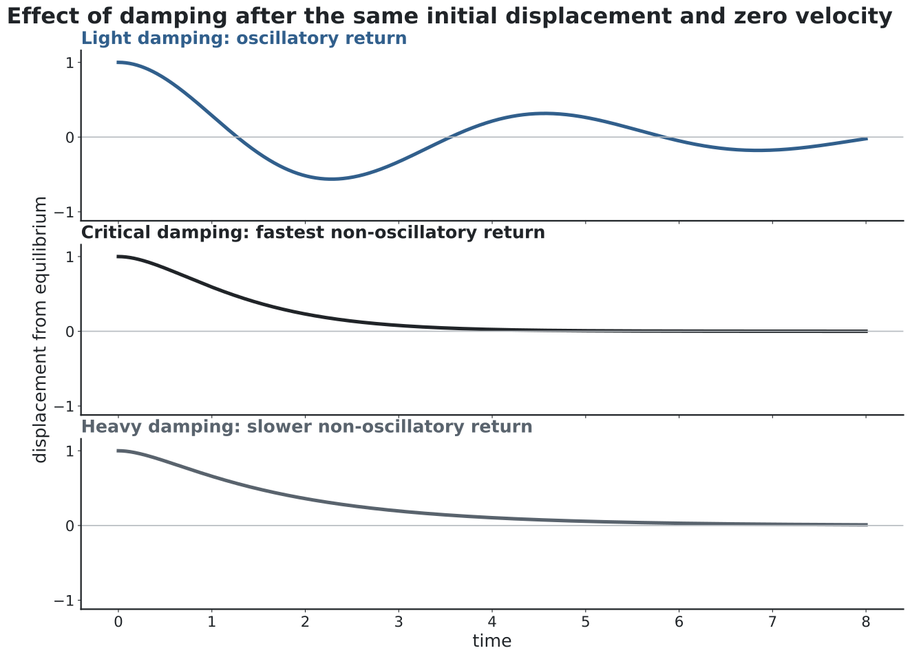
Figure: Starting from the same displacement and zero initial velocity, light damping gives repeated crossings with decreasing amplitude, critical damping gives the fastest non-oscillatory return, and heavy damping returns more slowly without oscillating.

If a periodic external force acts on a system in one dimension:

$$F(t)=F_0\cos {\omega }_{d}t$$

where ${\omega }_d$ is the driving angular frequency. The system undergoes forced oscillation. At steady state, it oscillates at the driving frequency.

Resonance occurs when the driving frequency $f_{\text{d}}=\frac{{\omega }_d}{2\pi }$ is close to the natural frequency:

$$f_{\text{d}}\approx f_0$$

Greater damping causes a lower, broader resonance peak. See Damping and Resonance.

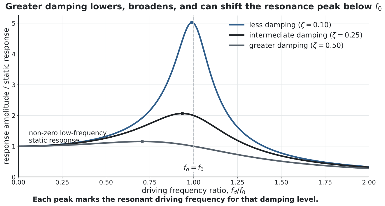
Figure: Increasing damping lowers and broadens the displacement-amplitude response. The maximum occurs at $f_r$ near $f_0$ for light damping and can shift below $f_0$ as damping increases.

Enrichment — Circular Motion Connection

Enrichment — not an explicit 9749 Oscillations learning outcome

The projection model is a useful way to visualise the sinusoidal solution and phase, but it is not required as a separate 9749 Oscillations outcome.

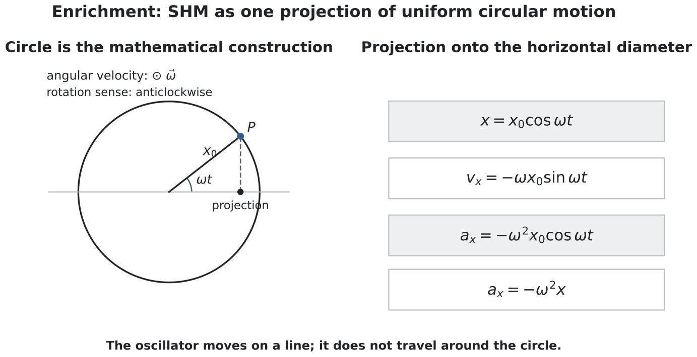
Figure: As a point moves uniformly around a circle, its projection onto one diameter has displacement $x=x_0\cos \omega t$ and acceleration $a_x=-{\omega }^{2}x$. The circle is a mathematical representation, not the path of the oscillator itself.

The projection of uniform circular motion onto a diameter gives SHM. If a particle moves in a circle of radius $r$ with angular velocity vector $\vec{\omega }$ (conventionally anti-clockwise to be positive), its angular speed is $\omega =|\vec{\omega }|$. Then the projections on the coordinate axes are:

$$x=r\cos \omega t$$ $$y=r\sin \omega t$$

So SHM can be viewed as the one-dimensional projection of uniform circular motion onto either the $x$- or $y$-axis.

Problem-Solving Checklist

If given period:

$$f=\frac{1}{T},\omega =\frac{2\pi }{T}$$

If given amplitude and position:

$$v=\pm \omega \sqrt{x_0^2-x^2}$$

If asked whether motion is SHM, check whether:

$$\vec{a}\propto -\vec{x}$$

or in one-dimensional signed form:

$$a\propto -x$$

If energy is involved:

$$E_T=\frac{1}{2}m{\omega }^2{x}_0^2$$

Exam Relevance

Common exam tasks include:

• stating the SHM definition and explaining the negative sign;
• using $a=-{\omega }^{2}x$ in one-dimensional signed problems;
• interpreting $x$-$t$, $v$-$t$, $a$-$t$, $a$-$x$, and energy graphs;
• applying $a=-{\omega }^{2}x$ to spring, pendulum, or unfamiliar restoring-force contexts;
• explaining why a pendulum formula requires small angles;
• comparing damping types;
• explaining resonance curves and practical resonance examples.

Common mistakes:

• forgetting the negative sign in $a=-{\omega }^{2}x$;
• confusing amplitude with instantaneous displacement;
• using the pendulum formula for large angles;
• forgetting velocity is zero at turning points;
• assuming resonance is always beneficial.

Summary

Quantity	Expression
Frequency	$f=1/T$
Angular frequency	$\omega =2\pi f$
SHM condition	$a=-{\omega }^{2}x$
Displacement	$x=x_0\sin (\omega t+{\varphi }_0)$
Velocity	$v=\omega x_0\cos (\omega t+{\varphi }_0)$
Max speed	$v_{\max }=\omega x_0$
Max acceleration	$a_{\max }={\omega }^2{x}_0$
Total energy	$\frac{1}{2}m{\omega }^2{x}_0^2$
Spring period	$2\pi \sqrt{m/k}$
Pendulum period	$2\pi \sqrt{l/g}$

Links

• Prerequisite: Kinematics
• Prerequisite: Forces
• Prerequisite: Work, Energy and Power
• Related: Circular Motion
• Related: Waves
• Branch: Simple Harmonic Motion
• Branch: Spring Motion
• Branch: Floating Object SHM
• Branch: Damping and Resonance
• Branch: Pendulum Motion
• Concept: Phase Difference

Provenance

• source file: Oscillation Lecture Anchor Notes
• generated by: bridging_tools/ingest_JC_phy_wiki.py
• manifest entry: content/topics/09_oscillations_and_simple_harmonic_motion/resources/Oscillation_Lecture_Anchor_Notes.pdf
• source hash: b21f19dd5702c1868bffa66ed50a27d4edbf80149c2c5b2daeafc268d642185c