AC Generator Waveforms

Overview

This note connects coil orientation, magnetic flux linkage $\lambda =N\Phi$, and induced emf $\mathcal{E}$. The reliable method is to declare the angle and polarity convention, write $\lambda (t)$, and then use Faraday’s law.

Core Ideas

• Flux linkage describes magnetic flux through all turns of the coil.
• Emf is the negative time derivative of flux linkage.
• Flux-linkage extrema correspond to zero emf.
• Flux-linkage zero crossings correspond to maximum emf magnitude for uniform rotation.
• The quarter-cycle relation follows from differentiation, while the sign depends on the reference polarity.

Convention used here

Let $\theta$ be the angle between $\mathbf{B}$ and the coil normal $\hat{\mathbf{n}}$. At $t=0$:

• $\hat{\mathbf{n}}$ is parallel to $\mathbf{B}$;
• $\theta =0$;
• $\lambda =+NBA$;
• the chosen emf is initially zero and then positive.

For uniform rotation,

$$\theta =\omega t=\frac{2\pi t}{T}.$$

Analytical waveforms

The flux linkage is

$$\lambda =NBA\cos \omega t.$$

Faraday’s law gives

$$\begin{array}{rl}\mathcal{E}& =-\frac{\mathrm{d}\lambda }{\mathrm{d}t}\\ & =NBA\omega \sin \omega t.\end{array}$$

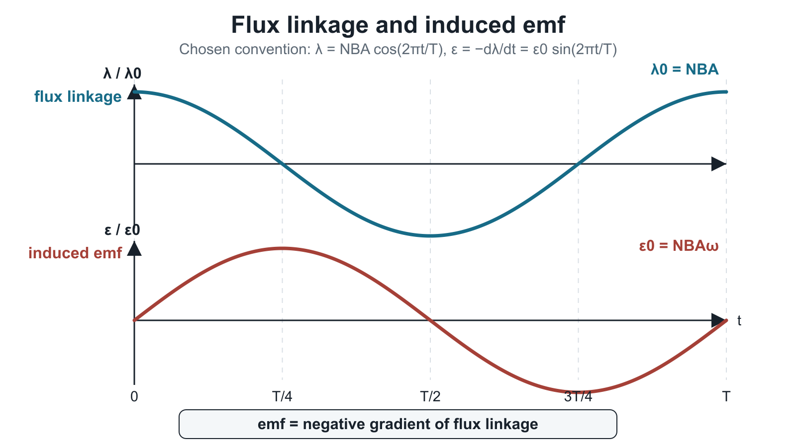
Figure: The cosine flux-linkage curve and sine emf curve under one declared convention. Dashed guides align the quarter-turns. The emf sign is opposite to the flux-linkage gradient.

Gradient reasoning

At a maximum or minimum of $\lambda$,

$$\frac{\mathrm{d}\lambda }{\mathrm{d}t}=0,$$

so $\mathcal{E}=0$.

At a zero crossing, $|\mathrm{d}\lambda /\mathrm{d}t|$ is greatest, so $|\mathcal{E}|$ is greatest.

The sign follows directly:

• decreasing $\lambda$ gives a negative gradient and positive chosen $\mathcal{E}$;
• increasing $\lambda$ gives a positive gradient and negative chosen $\mathcal{E}$.

This is safer than memorising “lead” or “lag” without a convention.

Quarter-turn map

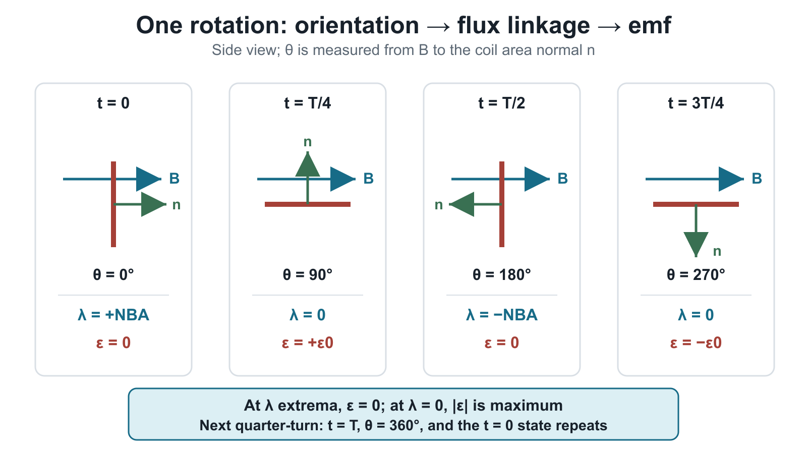
Figure: Coil positions and waveform values at successive quarter-turns. The area vector is parallel to $\mathbf{B}$ at maximum positive flux linkage and antiparallel at maximum negative flux linkage. At the edge-on positions, flux linkage is zero and emf magnitude is maximum.

Rotation	$\lambda$	Gradient of $\lambda$	$\mathcal{E}$
$0^{\circ }$	$+NBA$	$0$	$0$
$90^{\circ }$	$0$	most negative	$+{\mathcal{E}}_0$
$180^{\circ }$	$-NBA$	$0$	$0$
$270^{\circ }$	$0$	most positive	$-{\mathcal{E}}_0$
$360^{\circ }$	$+NBA$	$0$	$0$

Phase language used carefully

With

$$\lambda =NBA\cos \omega t$$

and

$$\mathcal{E}={\mathcal{E}}_0\sin \omega t,$$

the cosine flux-linkage waveform is one quarter-cycle ahead of the sine emf waveform in the usual time-shift description. Reversing the emf reference polarity changes the sine sign. Therefore, graph landmarks and gradient reasoning are more robust than an isolated “leads by $90^{\circ }$” statement.

Effects of angular speed

For fixed $N$, $B$ and $A$,

$$\mathcal{E}(t)=NBA\omega \sin \omega t.$$

Angular speed sets both the peak emf and the rate of phase change.

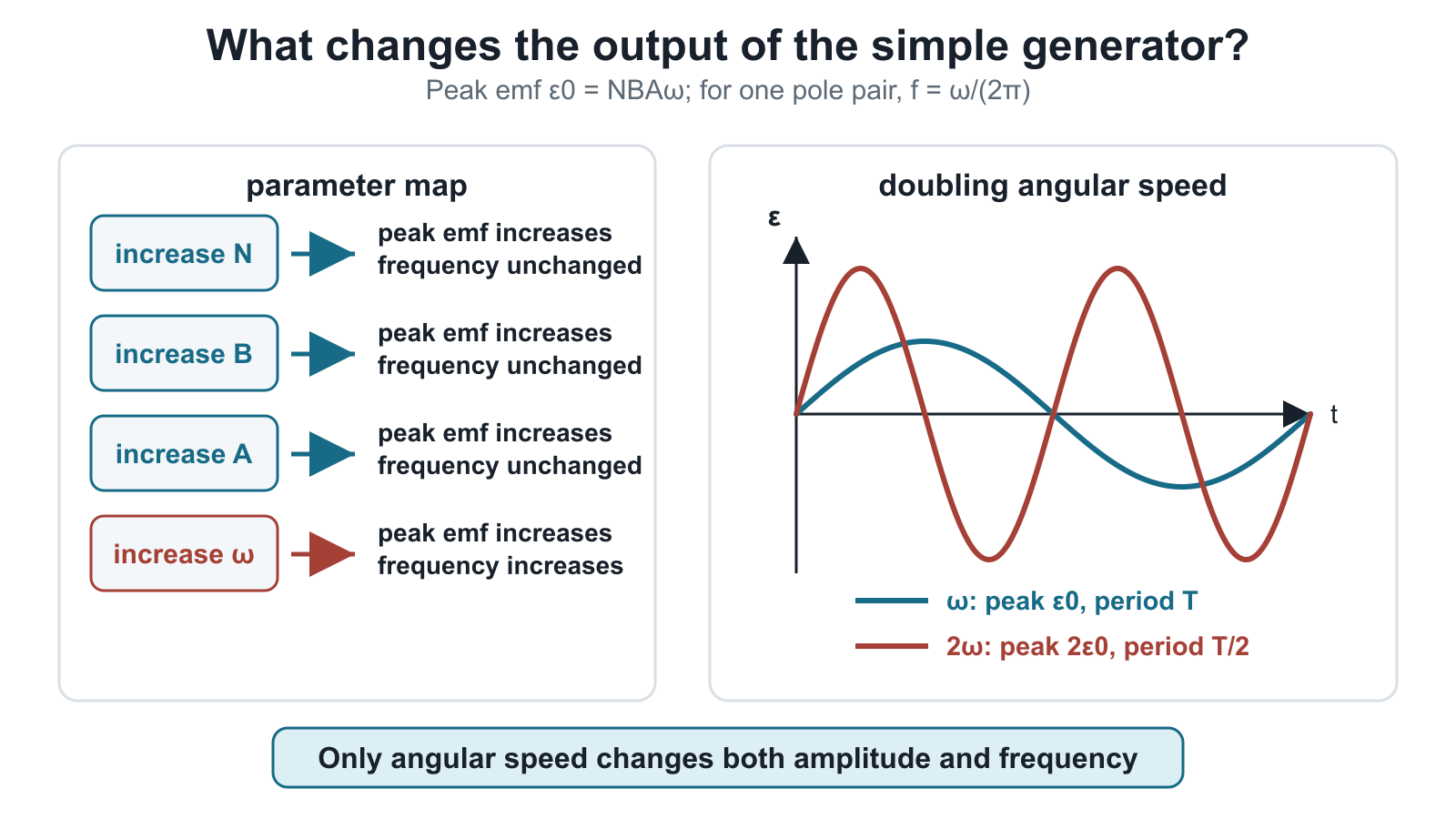
Figure: $N$, $B$ and $A$ scale peak emf only. When angular speed doubles, peak emf doubles and two cycles occur in the time previously required for one.

Worked Example 1: infer emf from flux linkage

Suppose $\lambda$ is at its maximum positive value and begins to decrease at $t=0$.

• At $t=0$, its gradient is zero, so $\mathcal{E}=0$.
• At $T/4$, it crosses zero with its most negative gradient, so $\mathcal{E}=+{\mathcal{E}}_0$ under this convention.
• At $T/2$, it is minimum and momentarily not changing, so $\mathcal{E}=0$.

If the flux-linkage graph instead crosses zero upward, its gradient is positive and therefore $\mathcal{E}<0$ for the same polarity convention.

Worked Example 2: instantaneous emf

A generator has peak emf $120\mathrm{V}$ and frequency $50\mathrm{Hz}$. If its emf starts from zero and increases,

$$\mathcal{E}=120\sin (2\pi \times 50t).$$

At $t=2.5\mathrm{ms}$,

$$\mathcal{E}=120\sin \left(2\pi \times 50\times 2.5\times 10^{-3}\right)=84.9\mathrm{V}.$$

Worked Example 3: rotational speed

In the simple one-pole-pair model, a coil rotates at $25\mathrm{rev}{\mathrm{s}}^{-1}$. One revolution gives one cycle, so

$$f=25\mathrm{Hz},\omega =2\pi f=50\pi \mathrm{rad}{\mathrm{s}}^{-1}.$$

Quick graph-sketch method

1. Mark $0$, $T/4$, $T/2$, $3T/4$ and $T$.
2. Plot flux-linkage values from the coil orientation.
3. Inspect the flux-linkage gradient at each time.
4. Plot $\mathcal{E}$ with the opposite sign to that gradient.
5. Check that the ideal sinusoidal emf has zero mean over a complete cycle.

Common Mistakes

• drawing identical flux-linkage and emf graphs;
• using $\Phi$ when $N\Phi$ is required;
• forgetting the negative derivative when assigning polarity;
• treating $NBA\omega$ as the emf at every time;
• confusing $f$ with $\omega$;
• changing amplitude but not frequency when $\omega$ changes.

Exam Relevance

Waveform questions often award marks for connecting coil orientation, flux linkage and graph gradient. Declare the angle and polarity convention before assigning signs, then show the quarter-period landmarks.

Links

• Alternating Current Generators
• Alternating Current Generators Common Exam Traps
• Electromagnetic Induction
• Alternating Current

Summary

Under the declared convention,

$$\lambda =NBA\cos \omega t,\mathcal{E}=NBA\omega \sin \omega t.$$

The emf is zero at flux-linkage extrema and has maximum magnitude at flux-linkage zero crossings.