Half-Life

Branch note: This page deepens one part of Nuclear Physics.

Overview

Half-Life describes how radioactive substances decrease with time. It is a statistical measure of radioactive decay and one of the most important tools for solving nuclear-decay problems.

This topic connects directly with:

• Radioactive Decay
• Nuclear Physics

Core Ideas

• half-life is the time for an undecayed quantity to fall to half its value
• individual nuclei decay randomly, but large samples behave predictably
• decay constant measures the probability of decay per unit time
• undecayed nuclei, activity, and corrected count rate all decay exponentially with the same half-life
• background count rate must be subtracted before using count-rate data for half-life analysis

Connection to Radioactive Decay

Radioactive nuclei decay:

• spontaneously
• randomly
• independently of one another

Although individual nuclei decay unpredictably, a large sample behaves in a predictable way.

That predictable decrease gives rise to the idea of half-life.

Definition of Half-Life

The half-life of a radioactive nuclide is the time taken, for that nuclide, for:

• the number of undecayed nuclei to fall to half its original value

or equivalently:

• activity to fall to half its original value
• corrected count rate to fall to half its original value

Symbol:

$$t_{1/2}$$

Half-life is not the time for a sample to disappear. In equal half-life intervals, the same fraction of the remaining sample decays, not the same fixed amount.

Random Decay and Statistical Predictability

Individual Nucleus

It is impossible to know exactly when one nucleus will decay.

Large Sample

For many nuclei:

• average behaviour is highly predictable
• the sample follows the exponential decay law

This is why half-life is meaningful and measurable.

Decay Constant Overview

The decay constant is:

$$\lambda$$

It represents the probability per unit time that a nucleus decays.

Unit:

$${\text{s}}^{-1}$$

Larger $\lambda$ means:

• faster decay
• shorter half-life

For a sufficiently short interval $\Delta t$, the probability that one undecayed nucleus decays is approximately $\lambda \Delta t$. For $N$ undecayed nuclei, the expected decrease is

$$\Delta N\approx -\lambda N\Delta t.$$

Taking the rate limit gives

$$\frac{dN}{dt}=-\lambda N.$$

The negative sign describes the decrease in the number remaining. Individual counts fluctuate around this expectation; the equation describes the mean behaviour of a large ensemble.

Half-Life Relation

$$t_{1/2}=\frac{\ln 2}{\lambda }$$

Therefore:

• large $\lambda$ gives small half-life
• small $\lambda$ gives long half-life

Decay Law Overview

Number of Undecayed Nuclei

$$N=N_0{e}^{-\lambda t}$$

where:

• $N_0$ = initial number
• $N$ = number remaining after time $t$

Activity

Since activity is proportional to the number of undecayed nuclei:

$$A=-\frac{dN}{dt}=\lambda N$$

and:

$$A=A_0{e}^{-\lambda t}$$

Count Rate

Activity is the true decay rate of the source. A detector count rate is normally smaller because the detector subtends only part of the emitted radiation and is not perfectly efficient.

If detector geometry, detector efficiency and absorption between source and detector remain constant, the corrected source count rate is proportional to activity and follows:

$$C=C_0{e}^{-\lambda t}$$

where:

• $C_0$ = initial corrected source count rate
• $C$ = corrected source count rate at time $t$

Undecayed nuclei, activity, and corrected count rate follow the same exponential decay shape.

Repeated Halving Method

After each half-life, the quantity halves.

Time	Remaining Fraction
$0$	$1$
$t_{1/2}$	$\frac{1}{2}$
$2t_{1/2}$	$\frac{1}{4}$
$3t_{1/2}$	$\frac{1}{8}$
$4t_{1/2}$	$\frac{1}{16}$

This is useful when the time is an exact multiple of the half-life.

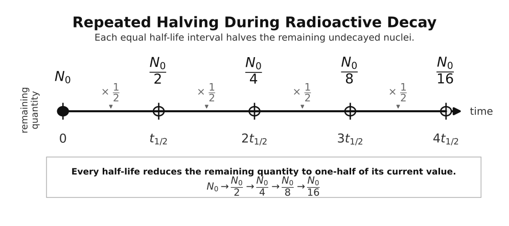
Figure: Equal half-life intervals halve the remaining radioactive quantity each time. The absolute amount that decays becomes smaller each interval because the same fraction, not the same number of nuclei, decays.

Activity, Count Rate and Nuclei Linkage

These three quantities are proportional:

• undecayed nuclei $N$
• activity $A$
• corrected count rate $C$

So they all fall with the same half-life.

Here, corrected count rate means the source count rate after background count rate has been subtracted.

If $N$ halves:

• $A$ halves
• corrected $C$ halves

Background Count Overview

A detector records background radiation even when the named source is absent. Natural sources include cosmic radiation, rocks, soil, radon and radioactive materials in the environment; medical and other human-made sources may also contribute.

Measured count rate:

$$C_{\text{measured}}=C_{\text{source}}+C_{\text{background}}$$

Therefore:

$$C_{\text{source}}=C_{\text{measured}}-C_{\text{background}}$$

Always subtract the mean background rate before using count-rate data to determine half-life. Because background counts are random too, estimate their mean with the source removed and over a sufficiently long counting time.

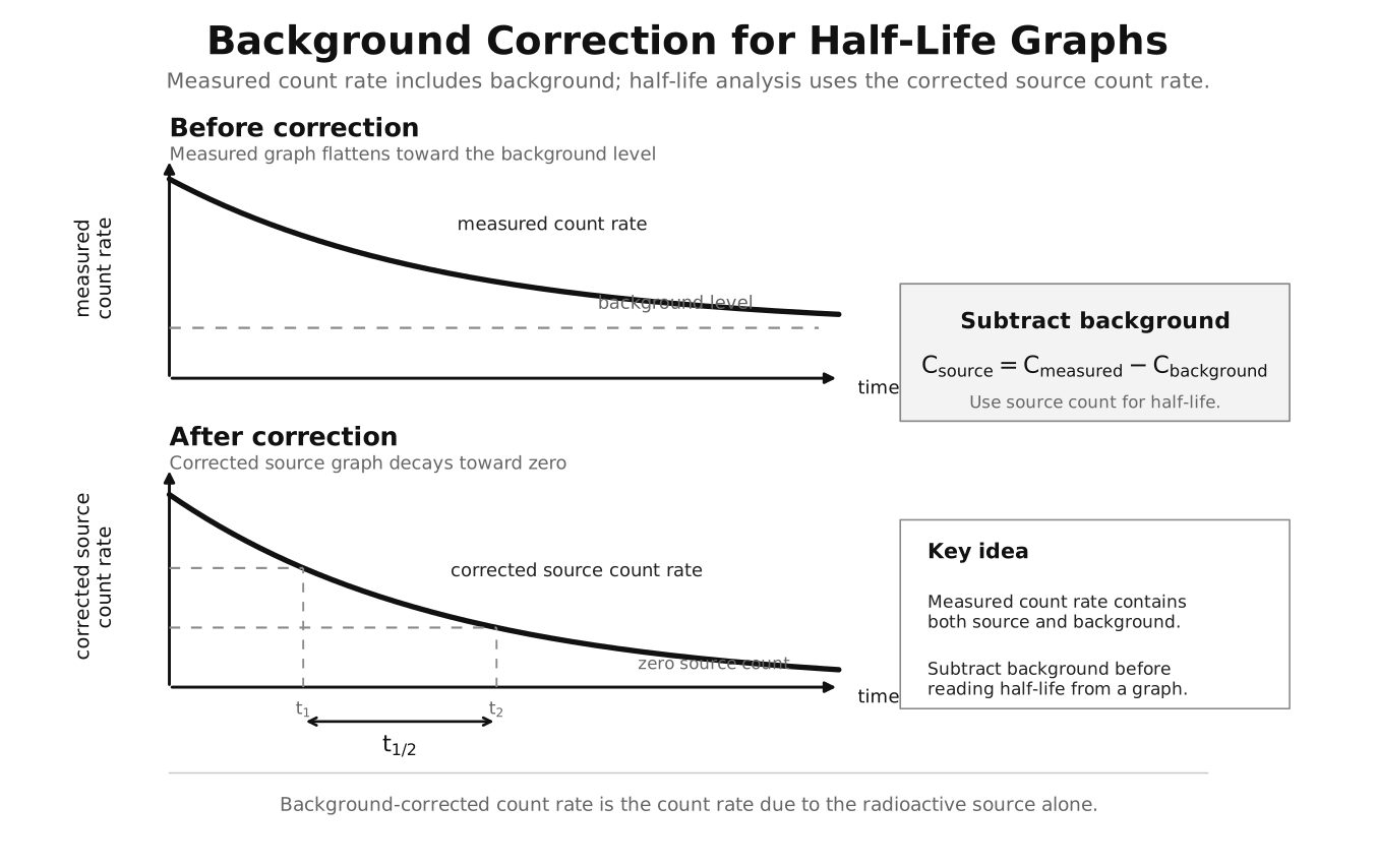
Figure: The measured count rate approaches the non-zero background rate, whereas the corrected source count rate approaches zero. Subtract the mean background rate first, then read half-life from equal successive halvings of the corrected curve. Corrected count rate is proportional to source activity only while detector geometry, detector efficiency and intervening absorption remain unchanged.

Graph Overview

Decay graphs of:

• $N$ against $t$
• $A$ against $t$
• $C$ against $t$

are exponential curves:

• steep at first
• flatten gradually
• approach zero asymptotically in the ideal continuous model

The smooth exponential curve represents an ensemble expectation or continuous model and therefore does not reach zero at a finite time. A real finite sample contains a discrete number of nuclei and can eventually contain zero undecayed nuclei. Measured count-rate graphs flatten towards the background count, while corrected source count-rate graphs flatten towards zero in the ideal model.

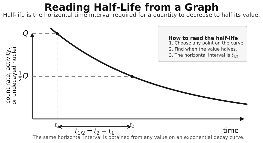
Figure: Half-life is the horizontal time interval for a decay graph to fall from any value to half that value. Repeating the reading at lower count rates should give the same half-life for the same nuclide, apart from experimental scatter.

See Exponential Decay and Graphs.

Short Worked Examples

Example 1: Repeated Halving

Half-life = 5 h

Initial activity = 800 Bq

After 15 h:

• 3 half-lives

$$800\to 400\to 200\to 100$$

Answer:

$$100\text{Bq}$$

Example 2: Find Half-Life

A sample drops from 1200 Bq to 300 Bq in 8 h.

$$1200\to 600\to 300$$

So there are two half-lives in 8 h.

Therefore:

$$t_{1/2}=4\text{h}$$

Example 3: Background Count

Measured count rate = 90 counts min${}^{-1}$

Background count rate = 15 counts min${}^{-1}$

Corrected source count rate:

$$90-15=75$$

Use 75 for decay calculations.

Example 4: Half-Life from Raw Detector Readings

A detector measures $215\mathrm{counts}\mathrm{mi}{\mathrm{n}}^{-1}$ initially and $65\mathrm{counts}\mathrm{mi}{\mathrm{n}}^{-1}$ after $8.0\mathrm{h}$. The mean background is $15\mathrm{counts}\mathrm{mi}{\mathrm{n}}^{-1}$.

Correct both readings:

$$C_{0,\mathrm{source}}=215-15=200\mathrm{counts}\mathrm{mi}{\mathrm{n}}^{-1},$$ $$C_{\mathrm{source}}=65-15=50\mathrm{counts}\mathrm{mi}{\mathrm{n}}^{-1}.$$

The source rate has fallen from $200$ to $100$ to $50$: two half-lives occur in $8.0\mathrm{h}$. Therefore

$$t_{1/2}=\frac{8.0}{2}=4.0\mathrm{h}.$$

Using the uncorrected readings would give a wrong ratio because the background does not decay with the source.

Exam Relevance

Students should be able to:

• define half-life correctly for undecayed nuclei, activity, and corrected count rate
• distinguish random single-nucleus behaviour from predictable large-sample behaviour
• use repeated halving for simple calculations
• use exponential-decay relations and the half-life formula
• correct count-rate data for background before analysing graphs

Formula Sheet

Decay Law

$$N=N_0{e}^{-\lambda t}$$

Activity

$$A=-\frac{dN}{dt}=\lambda N$$

Activity Decay

$$A=A_0{e}^{-\lambda t}$$

Count Rate Decay

$$C=C_0{e}^{-\lambda t}$$

Half-Life Relation

$$t_{1/2}=\frac{\ln 2}{\lambda }$$

Common Exam Traps Overview

Students often confuse:

• half-life with complete disappearance
• random single decay with predictable sample decay
• activity with the number decayed
• measured count rate with corrected count rate
• repeated-halving steps
• the units and meaning of $\lambda$
• treating the smooth exponential curve as the exact result of every short counting interval rather than the ensemble mean

See Half-Life Common Exam Traps.

Quick Revision Summary

• half-life is the time for a quantity to halve
• it applies to $N$, $A$, and corrected $C$
• radioactive decay is random for one nucleus but predictable for many
• decay follows the exponential law
• larger decay constant means shorter half-life
• subtract background count before analysis

Links

• Radioactive Decay
• Nuclear Physics
• Exponential Decay and Graphs
• Half-Life Common Exam Traps